
System of Delayed Differential Equations
A system of Delayed Differential Equations (DDEs) was constructed to model the kinetics of the different proteins and their interaction. This model was used to figure out how we can expect the initial genetic circuit to behave. Predicting the behaviour of the model was important in order to adjust the wet lab experiments. It was also used to shed light on how the system could react under different conditions.
Introduction
The oscillatory circuit consists of a receptor (RhlR) which can receive its cognate ligand (C4-HSL) to activate an inducible promoter (pRhl). An AHL synthase (RhlI) producing the cognate ligand is under the control of the inducible promoter, creating a positive feedback loop. Under the same promoter, a lactonase (AiiA) is also controlled, which degrades the cognate ligand, creating a negative feedback loop.
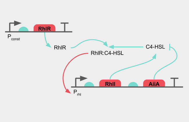
Figure 1: Diagram of the oscillatory system
The presence of C4-HSL together with RhlR activates pRhl, which produces more RhlI synthase, which in turn creates more C4-HSL. The positive feedback loop amplifies the C4-HSL signal until enough AiiA has been synthesised. As the lactonase starts degrading the C4-HSL, the signal decreases. The negative feedback loop decreases the C4-HSL signal until no new protein is produced and the remaining active protein is broken down.


Figure 2: Descriptive diagram of the oscillatory system. Click on the arrows to move between pictures.
Since there is a delay from a transcription factor to activate the transcription of a protein, for that protein to fold into its correct shape and then for it to acts its function, the system doesn't reach as stable equilibrium, but oscillates between a state where the positive and the negative feedback loop dominates. As AHL is a signal molecule and free to diffuse across membranes, the oscillation in not contained to one cell, but is synchronized to the entire population of cells, allowing for any gene controlled by the oscillator to be greatly amplified across the colony at the same time periods Danino et al., 2010.
The complete oscillatory circuit can be modelled with the following system of differential equations where C4-HSL is denoted "H" and the gene of interest, such as a reporter gene, is denoted "X".
$$ \frac{\partial [RhlI]}{\partial t} = \frac{V_{max,i}}{K_m \times [H]^2 } + \frac{V_{max,a} \times [H]^2}{K_m + [H]^2 } - \frac{V_{max,g} \times [RhlI]}{K_{g} + [RhlI] + [AiiA] + [X]} $$ $$ \frac{\partial [AiiA]}{\partial t} = \frac{V_{max,i}}{K_m + [H]^2 } + \frac{V_{max,a} \times [H]^2}{K_m + [H]^2 } - \frac{V_{max,g} \times [AiiA] }{K_{g} + [RhlI] + [AiiA] + [X]} $$ $$ \frac{\partial [X]}{\partial t} = \frac{V_{max,i}}{K_m + [H]^2 } + \frac{V_{max,a} \times [H]^2}{K_m + [H]^2 } - \frac{V_{max,g} \times [X]}{K_{g} + [RhlI] + [AiiA] + [X] } $$ $$ \frac{\partial [H]}{\partial t} = \frac{V_{max,H} \times [RhlI]}{K_H + [RhlI] } - \frac{k_{cat,g} \times [AiiA] \times [H]}{K_G+[AiiA]} $$
Each partial differential equation for change in protein concentration over time consists of three parts. The transcription of the uninduced pRhl promoter or the "leaky" transcription is here first in the equations. The activity of the uninduced promoter, sometimes denoted "a", or a0 O'Brien et al. 2010, here denoted "Vmax, i" is in the numerator, without any dependence on the inducer (AHL). It is also assumed that the receptor (RhlR) is present in excessive amounts, so this too is not found in this set of equations.
$$ \frac{V_{max,i}}{K_m \times [H]^2 } $$
The second part of the equation is the induced transcription of the promoter. This is a Hill function with a cooperativity of 2, by the binding mechanism of RhlR to the promoter Stricker et al., 2008.
$$ \frac{V_{max,a} \times [H]^2}{K_m + [H]^2 } $$
The third and final part is the degradation of the enzyme by the proteasome complex in the cell. The proteins in the circuit are all designed with an LVA tag, which is an ssRA tag that tags the protein for destruction. This causes the proteins to linger in the cell for shorter amounts of time, which is crucial for creating a fast oscillator. Slower repressilator circuits would have to resort to using the concentration drop in division to decrease protein levels Elowitz & Leibler., 2000. This is avoided by using a degradation tag. Since all of our proteins will be expressed on a high copy number plasmid, only our proteins are important in the denominator for the degradation complex. The protein "X" is here chosen for the example.
$$ - \frac{V_{max,g} \times [X]}{K_{g} + [RhlI] + [AiiA] + [X] } $$
The equation for the AHL is different as it is a small molecule made by the enzyme RhlI. It is therefore in the first part dependent on the concentration of RhlI in the cell.
$$ \frac{V_{max,H} \times [X]}{K_H + [X] } $$
It is also actively broken down by AiiA, which is dependent on both the concentration of AiiA and the current concentration of AHL, which can be seen in the second part of the equation.
$$ - \frac{k_{cat,g} \times [AiiA] \times [H]}{K_G+[AiiA]} $$
With a system of ODEs, the delay caused by transcription, translation and folding can be modelled by introducing intermediate species for the mRNA, the unfolded protein and the different folding species, each with their own enzymatic activity. While this provides a simulation with high external validity, it requires the kinetic parameters for the transition of one species to another, and with the partially folded proteins: their enzymatic activity as well Stricker et al., 2008. A simpler approach is to summarize all the interactions that have to occur before a protein is active with a time delay from induction of the gene to the final protein. This can be done with a system of DDEs, with the following additional equation that introduces the time delay. While this may not be as powerful at predicting experimental outcomes, it is easier to construct and uses less unknown variables O'Brien et al. 2010. This changes the system of equations from a set of ODEs, to DDEs. These are significantly harder to solve analytically, and we have therefore resorted to solving them numerically in MATLAB.
$$ \frac{\partial [RhlI]}{\partial t} = \frac{V_{max,i}}{K_m \times [H_{t-\tau}]^2 } + \frac{V_{max,a} \times [H_{t-\tau}]^2}{K_m + [H_{t-\tau}]^2 } - \frac{V_{max,g} \times [RhlI]}{K_{g} + [RhlI] + [AiiA] + [X]} $$ $$ \frac{\partial [AiiA]}{\partial t} = \frac{V_{max,i}}{K_m + [H_{t-\tau}]^2 } + \frac{V_{max,a} \times [H_{t-\tau}]^2}{K_m + [H_{t-\tau}]^2 } - \frac{V_{max,g} \times [AiiA] }{K_{g} + [RhlI] + [AiiA] + [X]} $$ $$ \frac{\partial [X]}{\partial t} = \frac{V_{max,i}}{K_m + [H_{t-\tau}]^2 } + \frac{V_{max,a} \times [H_{t-\tau}]^2}{K_m + [H_{t-\tau}]^2 } - \frac{V_{max,g} \times [X]}{K_{g} + [RhlI] + [AiiA] + [X] } $$ $$ \frac{\partial [H]}{\partial t} = \frac{V_{max,H} \times [RhlI]}{K_H + [RhlI] } - \frac{k_{cat,g} \times [AiiA] \times [H]}{K_G+[AiiA]} $$
The equations remain mostly the same, but the change in mature protein expression is now dependent not on the current level of AHL, but the level of AHL at a time point tau time ago.
Priming of the oscillations
Running the simulation with generic values for the kinetic parameters is useful to determine the general behaviour of the system. The first task was to see how just the oscillatory circuit presented in the previous paragraphs behaves. The simulation was run with both some initial amount of AHL, denoted "primed", and with no initial AHL, denoted "non-primed". The "primed" scenario is supposed to represent a system where AHL from surrounding cells enters the population in question, or when the oscillation is kickstarted by addition of AHL into the culture. The "non-primed" scenario is when the culture is left to itself, without any external stimulus from the researchers or other cells.


Figure 3: Basic oscillatory circuit. Concentrations of RhlI (I), AiiA (A), MtrB (X) and C4-HSL (H) plotted over time
The simulation shows that oscillations are indeed possible with this circuit. The oscillations start immediately when "primed", but take longer to form when not "primed". The leaky transcription is eventually enough to start the positive feedback loop, which starts the oscillations of the system. Since the culture is going to remain for some time, it can therefore be concluded that oscillations will start eventually, regardless of whether the initial AHL is present or not. Future simulations will however be "primed" with initial AHL. This conclusion does however eliminate any future system where the oscillations would be activated by an initial burst of the same AHL (in this case, the cognate AHL is C4-HSL) as the oscillations start regardless.
Initial design and induction
The second step is to create a system that can be induced. The initial design was to integrate a key part of the oscillatory circuit (RhlR) under an inducible promoter, and have the reporter gene under the pRhl promoter. The reporter gene in the final circuit would be MtrB, which in the knockout strain of Shewanella oneidensis would complete the Mtr complex and allow it to produce electricity. While independently developed, this initial design is similar to the one used by the 2015 NYMU iGEM team. NYMU-Taipei 2015
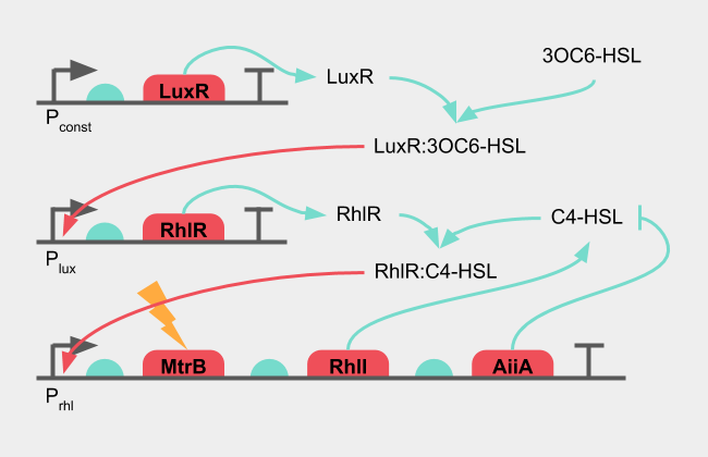
Figure 4: Diagram of the initial design of the oscillatory system
The inducible promoter would be the pLux promoter, which together with LuxR can receive 3OC6-HSL from E. coli. When there is no 3OC6-HSL present in the sample, there should be no induction of pLux, which in turn would result in no transcription of RhlR. The oscillatory circuit is then incomplete and should not produce any signal. The RhlR concentration here is not static, but requires its own equation. The reporter gene "X" remains under the control of pRhl, but the induction of the pRhl promoter gains another term: the concentration of RhlR. The 3OC6-HSL concentration receives the notation "H2" The set of DDEs then becomes the following.
$$ \frac{\partial [RhlI]}{\partial t} = \frac{V_{max,i}}{K_m \times [H_{t-\tau}]^2 } + \frac{V_{max,a} \times [RhlR] \times [H_{t-\tau}]^2}{K_m + [H_{t-\tau}]^2 } - \frac{V_{max,g} \times [RhlI]}{K_{g} + [RhlI] + [AiiA] + [X]} $$ $$ \frac{\partial [AiiA]}{\partial t} = \frac{V_{max,i}}{K_m + [H_{t-\tau}]^2 } + \frac{V_{max,a} \times [RhlR] \times [H_{t-\tau}]^2}{K_m + [H_{t-\tau}]^2 } - \frac{V_{max,g} \times [AiiA] }{K_{g} + [RhlI] + [AiiA] + [X]} $$ $$ \frac{\partial [X]}{\partial t} = \frac{V_{max,i}}{K_m + [H_{t-\tau}]^2 } + \frac{V_{max,a} \times [RhlR] \times [H_{t-\tau}]^2}{K_m + [H_{t-\tau}]^2 } - \frac{V_{max,g} \times [X]}{K_{g} + [RhlI] + [AiiA] + [X] } $$ $$ \frac{\partial [RhlR]}{\partial t} = \frac{V_{max,i}}{K_m + [H_{2,t-\tau}]^2 } + \frac{V_{max,a} \times [H_{2,t-\tau}]^2}{K_m + [H_{2,t-\tau}]^2 } - \frac{V_{max,g} \times [RhlR]}{K_{g} + [RhlR] } $$ $$ \frac{\partial [H]}{\partial t} = \frac{V_{max,H} \times [RhlI]}{K_H + [RhlI] } - \frac{k_{cat,g} \times [AiiA] \times [H]}{K_G+[AiiA]} $$
The simulation was run with different induction points, that is different timepoints at which the 3OC6-HSL (H2) was added to the system.


Figure 5: Initial inducible oscillatory circuit at different induction points of 3OC6-HSL. Concentrations of RhlI (I), AiiA (A), MtrB (X), C4-HSL (H), 3OC6-HSL (H2) and LuxR (R) plotted over time
When 3OC6-HSL is added to the system, the levels of RhlR rises to operational levels and the oscillations start. This is as desired from the design of the circuit. However, when the induction time point is moved, the oscillations start with the same offset. The phase of oscillation is dependent on when the induction happens.
This could pose a problem in large populations or large volumes where the transmission of the 3OC6-HSL signal might be diffusion limited. Some cells would encounter the signal before others, and initiate their oscillations before others. The system is not synchronized, which might lead to destructive interference and noise. Another circuit setup for inducing the electric signal would have to be made.
Improved design and induction
The mistake of the initial design was to put the reporter gene "X", or in our case: MtrB, under the same promoter as the oscillation. A solution to this synchronization problem is to have one part of a two-component induction oscillate, while the other depends on the signal received from E. coli. The LuxR, 3OC6-HSL pair to induce the pLux promoter can work as an AND-gate, where it will only initiate transcription downstream of pLux when both 3OC6-HSL and LuxR are present.
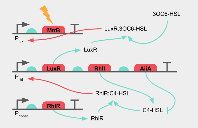
Figure 6: Diagram of the improved design of the oscillatory system
This does not require any new genes in the system, but simply a rearrangement, where LuxR is placed under oscillation, and MtrB under the pLux promoter. The system of equations in this improved system is the following.
$$ \frac{\partial [RhlI]}{\partial t} = \frac{V_{max,i}}{K_m \times [H_{t-\tau}]^2 } + \frac{V_{max,a} \times [H_{t-\tau}]^2}{K_m + [H_{t-\tau}]^2 } - \frac{V_{max,g} \times [RhlI]}{K_{g} + [RhlI] + [AiiA] + [LuxR]+ [X]} $$ $$ \frac{\partial [AiiA]}{\partial t} = \frac{V_{max,i}}{K_m + [H_{t-\tau}]^2 } + \frac{V_{max,a} \times [H_{t-\tau}]^2}{K_m + [H_{t-\tau}]^2 } - \frac{V_{max,g} \times [AiiA] }{K_{g} + [RhlI] + [AiiA] + [LuxR]+ [X]} $$ $$ \frac{\partial [LuxR]}{\partial t} = \frac{V_{max,i}}{K_m + [H_{t-\tau}]^2 } + \frac{V_{max,a} \times [H_{t-\tau}]^2}{K_m + [H_{t-\tau}]^2 } - \frac{V_{max,g} \times [LuxR]}{K_{g} + [RhlI] + [AiiA] + [LuxR] + [X]} $$ $$\frac{\partial [X]}{\partial t} = \frac{V_{max,i}}{K_m + [H_{2,t-\tau}]^2 } + \frac{V_{max,a} \times [H_{2,t-\tau}]^2}{K_m + [H_{2,t-\tau}]^2 } - \frac{V_{max,g} \times [X]}{K_{g} + [RhlI] + [AiiA] + [LuxR] + [X]} $$ $$ \frac{\partial [H]}{\partial t} = \frac{V_{max,H} \times [RhlI]}{K_H + [RhlI] } - \frac{k_{cat,g} \times [AiiA] \times [H]}{K_G+[AiiA]} $$
The simulation was run with different induction points. The parameters remained the same as in the simulation with the initial design.


Figure 7: Improved inducible oscillatory circuit at different induction points of 3OC6-HSL. Concentrations of RhlI (I), AiiA (A), MtrB (X), C4-HSL (H), 3OC6-HSL (H2) and LuxR (R) plotted over time
The oscillations of the system are active from the beginning, but no significant level of MtrB ("X") is produced. This allows the cells to synchronize as the levels of C4-HSL ("H") is oscillating from the very start, regardless of 3OC6-HSL ("H2") signals. When 3OC6-HSL is added to the system, the levels of MtrB oscillates with the rest of the system at much higher levels.
This was chosen as the circuit to implement in the project.
Supplementary:
The generic simulation was run with the following parameters:
| Description | Variable | Value |
|---|---|---|
| Basal expression rate of promoter, "leakiness" | Vmax,i | 0.01 |
| Maximum expression rate of promoter | Vmax,a | 1 |
| Dissociation constant (protein) | Km | 1 |
| Hills coefficient, "cooperativity" | h | 2 |
| Turnover of AHL by AiiA | kcat,G | 10 |
| Dissociation constant of AiiA | KG | 10 |
| Dissociation constant (synthase) | Vmax,H | 1 |
| Maximum protein degradation | KH | 0.5 |
| Dissociation constant for protein degradation | Vmax,g | 1.3 |
| Maximum expression rate of promoter | Kg | 0.5 |
Molecular Dynamics
Molecular dynamics computations were used in order to estimate the binding energy of several N-acyl homoserine lactones (AHLs) to AiiA. AHLs are targeted by lactonases such as AiiA (originally found in Bacillus thuringiensis), which hydrolases their lactone bond upon binding. This results in quenching of quorum sensing signaling. AutoDock Morris et al., 2019 was used to determine different binding positions and their respective docking energies. The conformation with the lowest binding energy was selected for comparison.
In these computations, we investigated the affinity of C4-HSL (noted HL4_ideal), C8-HSL (noted HTF), C6-oxo-HSL (noted HL6-ideal) for AiiA PDB entry 2a7m.
Because AiiA is a metalloenzyme containing two Zinc atoms the default autodock software does not assign any partial charge and is not appropriate (the Zn coordination sphere does not give explicit bonds, which is a problem for the algorithm), a tetrahedral Zn specific force field (with directional potentials) was used to modelize the enzyme Santos-Martins et al.,2014 instead of the default forcefield. The Lamarckian Genetic Algorithm was chosen as the docking algorithm, with a maximum of 2500000 energy evaluations. Molecular dynamics algorithms take into account the geometric constraints of both molecules and determine the best binding position by varying atoms' positions when possible and minimizing the free-energy of binding. The free-energy of binding is calculated thanks to an Amber force field by adding contributions that are intermolecular (Van der Waals, hydrogen bonds, desolvation and electrostatic energies) and intramolecular (torsional change in energy).
HL4-ideal
N-[(3S)-2-oxotetrahydrofuran-3-yl]butanamide
A grid centered on (12.736, 33.873, 28.824) was created, with 76 points in the x-direction, 72 in the y-direction and 58 in the z-direction. The distance between two points was 0,542Å.
The best binding position gave a free energy of binding of -5,06kcal/mol and inhibition constant of 195.69 μM at 298.15 K.
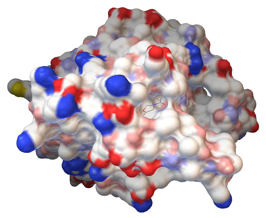
Figure 8: HL4-ideal in the binding pocket of AiiA
HL6-ideal
N-[(3S)-2-oxotetrahydrofuran-3-yl]hexanamide
A grid centered on (12.736, 33.873, 28.824) was created, with 112 points in the x-direction, 78 in the y-direction and 66 in the z-direction. The distance between two points was 0,386Å.
The best binding position gave a free energy of binding of -5,16kcal/mol and inhibition constant of 164,60 μM at 298.15 K.
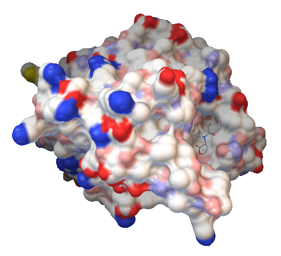
Figure 9: HL6-ideal in the binding pocket of AiiA
HTF-ideal
N-(2-oxotetrahydrofuran-3-yl)octanamide
A grid centered on (12.736, 33.873, 28.824) was created, with 112 points in the x-direction, 78 in the y-direction and 66 in the z-direction. The distance between two points was 0,386Å.
The best binding position gave a free energy of binding of -5.25 kcal/mol and inhibition constant of 140.75 μM at 298.15 K.
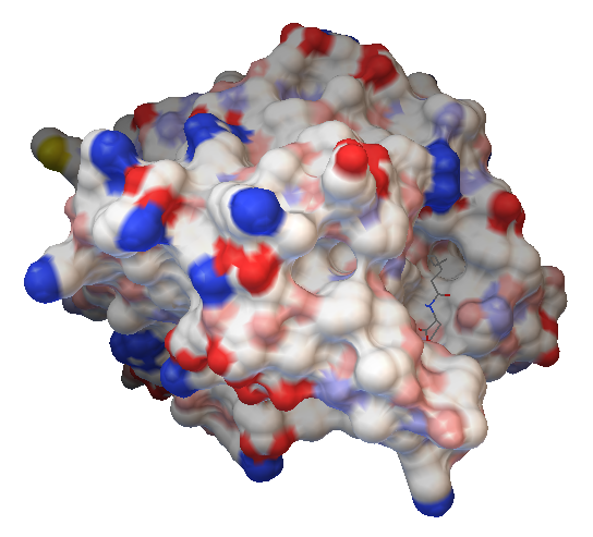
Figure 10: HTF-ideal in the binding pocket of AiiA
The binding energies and inhibition constants are summarized in Table 1 below. From this molecular dynamics analysis, we can conclude that there are crosstalks between different types of AHLs and AiiA, which might be a problem in our circuit given that both C6 and C4 are present. For further improvement, C4 could be modified so that its interactions with AiiA are improved and favored compared to other lactones. Another option would be to change the pair for other more specific molecules.
| C4 | C6 | C8 | |
|---|---|---|---|
| Binding energy (kcal/mol) | -5.06 | -5.16 | -5.25 |
| Inhibition constant (μM) | 195.69 | 164.60 | 140.75 |