Team:UESTC-Software/Model
<!DOCTYPE html>

Overview
We spend a lot of time and energy on building the model, which plays an important role in our project.
For domain surface shape feature extraction, the first step is to select the appropriate description method and feature extraction method. To implement this, we use the 3D Zernike descriptor[1] and the 3D-surfer website[2]. Through them, we have successfully obtained 121 dimensional data which can be used to describe the shape of domain surface. When clustering domain, a variety of clustering algorithms have been tested, and wefound that the traditional K-Means[3] algorithm is the best. After function statistics and screening, we extract functions that related to each domain, and selectively extract their function items by statistical methods. Combined with probability and statistics, the same statistical method is adopted to score the combination of different categories. For different model processing, thanks to Blender's powerful model processing ability and convenient code developing function, it impressively designed the original models as we want. By these methods, we have constructed a relatively complete database based on domain surface shape, which can provide new ideas and inspiration for biologists in protein synthesis.
Feature extraction
The three dimensional (3D) structure, especially the surface, plays a central role in various function of proteins. For example, a group in an active site on the 3D surface of the protein that carries outthe catalytic reaction of an enzyme.1 Further, surface residues on aninterface region establish physical contacts to another protein in protein–protein interactions.2,3 Therefore, classification of the 3D structureof proteins using an appropriate representation is critical for understanding the universe of protein structure, function, and evolution.
3D Zernike descriptor
The first step of computing 3D Zernike descriptor of a protein is to define the protein surface region in 3D space. To begin with, hetero atoms including water molecules in the PDB file of the target protein are removed. Then, the MSROLL program in Molecular Surface Package version 3.9.333 is used to compute the Connolly surface (triangle mesh) of the protein using default parameters. Next, the triangle mesh is placed in a 3D cubic gridof N3 (N 5 200), compactly fitting a protein to the grid. Each voxel (a cube defined by the grid) is assigned either1 or 0; 1 for a surface voxel that locates closer than 1.7grid interval to any triangle defining the protein surface,and 0 otherwise. Thus, the thickness of the protein surface is 3.4 grid intervals. The inside of a protein is keptempty so that 3D Zernike descriptor focuses on capturing the surface shape of a protein.
The method steps are as follows:
|
1. Voxelization of domain |
2. 3D Zernike transformation: The 3DZD program takes the cubic grid as input and generates 3DZDs (the 121 invariants). |
Firstly, to obtain 3D Zernike descriptors, one expands a given3D function f(x) into a series in terms of Zernike-Canterakis basis36 defined by the collection of functions
$Z^{m}_{nl}(r, \vartheta , \varphi)=R_{nl}(r)Y_{l}^{m}(\vartheta,\varphi)$
$Y_{l}^{m}(\vartheta , \varphi)=N_{l}^{m}P^{m}_{l}(cos\vartheta)e^{im\varphi}$
$N_{l}^{m}=\sqrt{\frac{2l+1}{4\pi}{\frac{(l-m)!}{{l+m}!}}}$
And Plm is the associated Legendre functions.Canterakis, constructed so that Znlm(r,W,u) are polynomials when writtenin terms of Cartesian coordinates as follows:The conversion between spherical coordinates and Cartesian x is defined as
$X=|X|\zeta=r\zeta=r(sin\vartheta sin\varphi,sin\vartheta cos\varphi, sin\varphi)^{T}$
Then the harmonics polynomials are defined as
$e_{l}^{m}(X)=r^{l}Y_{l}^{m}(\vartheta , \varphi)=r^{l}c_{l}^{m}(\frac{ix-y}{2})^{m}z^{l-m} \times \sum_{\mu=0}^{\lfloor \frac{l-m}{2} \rfloor} \bigl( \begin{smallmatrix} l\\ \mu \end{smallmatrix} \bigr) \bigl( \begin{smallmatrix} l-\mu \\ m+\mu \end{smallmatrix} \bigr) \bigl( \begin{smallmatrix} -\frac{x^{2}+y^{2}}{4z^{2}} \end{smallmatrix} \bigr)^{\mu}$
$c_l^{m}=c_l^{-m}=\frac{\sqrt{(2l+1)(l+m)!(l-m)!} }{l!}$
3D Zernike functions can be rewritten in Cartesian coordinates
$Z^{m}_{nl}(X)=R_{nl}(r)Y_{l}^{m}{\vartheta , \varphi} = \sum_{v=0}^{k}q^{v}_{kl}|X|^{2v}r^{l}Y^{m}_{l}( \vartheta , \varphi)= \sum_{v=0}^{k}q^{v}_{kl}|X|^{2v}e_{l}^{m}(X)$
To achieve rotation invariance
$q^{v}_{kl}=\frac{(-1)^{v}}{2^{2k}}\sqrt{\frac{2l+4k+3}{3}} \bigl( \begin{smallmatrix} 2k\\ k \end{smallmatrix} \bigr) (-1)^{v} \frac{ \bigl( \begin{smallmatrix} k\\ v \end{smallmatrix} \bigr) \bigl( \begin{smallmatrix} 2(k+l+v)+1\\ 2k \end{smallmatrix} \bigr) }{ \bigl( \begin{smallmatrix} k+l+v\\ k \end{smallmatrix} \bigr) }$
$\theta ^{m}_{nl} =\frac{3}{4 \pi} \int_{|x|\le 1} f(x)\bar{Z}^{m}_{nl}(X) \mathrm{d}x\ $
$F_{nl}=\sqrt{ \sum_{m=-l}^{m=l} {\Omega^{m}_{nl} }^{2}}$
Now that a protein 3D structure is represented by 121numbers, a comparison of two protein 3D structuressimply results in a comparison of two series of the 121numbers. we used three distance measuresfor comparing 3D Zernike descriptor of protein surfaceshapes. The first function is the Euclidean distance, dE,which is the RMSD of corresponding index numbers oftwo proteins:
$d_{E}=\sqrt{\sum_{i=0}^{i=nl}({Z_{Ai}-Z_{Bi})}^{2}}$
$d_{M}=\sum_{i=0}^{i=nl}|{Z_{Ai}-Z_{Bi}|}$
$d_{C}=1-Correlation Cofficient(Z_{A},Z_{B})$
3D Zernike descriptor and sphericalharmonic descriptor, the implementation formula is as follows.
3D-surfer website
This is a web-based tool designed to facilitate high-throughput comparison and characterization of proteins based on their surface shape. It provides us with a quick tool to compute 3D Zernike, which takes us only a few seconds to get the target descriptor.
Clustering Basis
Hopkins statistics
Clustering requires the data which are evenly distributed. Our data dimension is 121, which cannot be analyzed intuitively. Therefore, Hopkins statistics[4],a spatial statistic, is used to test the randomness of the spaceis.
$H=$$\frac{\sum_{i=1}^{n}y_{i}}{\sum_{i=1}^{n}x_{i}+\sum_{i=1}^{n}y_{i}}$
It can determine whether the data is evenly distributed, if so, clustering is not recommended. Close to 0 indicates the existence of clusters, close to 0.5 indicates the uniform distribution of data. Through this formula, we can illustrate whether clustering is reasonable.
We get the result: 0.14211. From the result, we can infer these 121 eigenvectors‘ similarity measure is based on distance, so we think clustering is a good choice.
Algorithm selection
Clustering algorithm comparison
In order to realize our clustering idea, we have tried many algorithms, such as SOM based on artificial neural networks, DBSCAN based on density, Mean Shift based on sliding window, K-means, etc. However, by comparing the clustering results and related evaluation indexes, we found that the traditional clustering algorithm K-means performed the best.
The first algorithm
SOM
A self-organizing map (SOM) is a type of artificial neural network (ANN) that is trained using unsupervised learning to produce a low-dimensional (typically two-dimensional), discretized representation of the input space of the training samples, called a map, and is therefore a method to do dimensionality reduction. Self-organizing maps differ from other artificial neural networks as they apply competitive learning as opposed to error-correction learning (such as backpropagation with gradient descent), and in the sense that they use a neighborhood function to preserve the topological properties of the input space.
Based on our sample capacity, the output layers are calculated as 31 by substituting into the formula.
Surprisingly, we repeating putting all kinds of two domains with similar shapes into SOM for prediction, but almost every time they are predicted as two types separately. Therefore, the result of clustering is bad.
The second algorithm
DBSCAN
Density-based spatial clustering of applications with noise (DBSCAN) is a data clustering algorithm proposed by Martin Ester, Hans-Peter Kriegel, Jörg Sander and Xiaowei Xu in 1996.[1] It is a density-based clustering non-parametric algorithm: given a set of points in some space, it groups together points that are closely packed together (points with many nearby neighbors), marking as outliers points that lie alone in low-density regions (whose nearest neighbors are too far away). DBSCAN is one of the most common clustering algorithms and also most cited in scientific literature.
After adjusting the parameters, we found that when the contour coefficient is very large, the number of clustering becomes very small. However, the contour coefficient becomes very small when the number of clustering is increased, so we gave up this algorithm.
The third algorithm
Mean Shift
Mean shift clustering is an algorithm based on sliding window to find the dense region of data points. The centroid-based algorithm locates the centroids of each group/type by updating the candidates for the centroids to the mean of the points in the sliding window.Then similar Windows are removed to form the center point set and corresponding grouping.
We found that the parameters for the best results are:r = 4, number of clusters: 673 and silhouette coefficient: - 0.1176.
The value of silhouette coefficient is negative, indicating poor clustering effect (The introduction of silhouette coefficient will be explained below. At the same time, because the Mean Shift algorithm adopts the greed rule, the number of types at the front is much larger than that at the back types, which is not conducive to our subsequent work on domain combining probability and functional statistics.
Kmeans
Overview of algorithms
K-Means algorithm is an unsupervised classification algorithm, assuming there are unlabeled data sets:
$X=\left[\begin{array}{c} x^{(1)}\\ x^{(2)}\\ \vdots\\ x^{(m)} \end{array}\right]$
The task of this algorithm is to gather the data into $k$ intoclusters $C=C_{1},C_{2},\ldots,C_{k}$,and the Minimum loss function is:
$E=\sum \limits_{i=1}^{k}\sum\limits_{x\in C_{i}}\parallel x-\mu_{i}\parallel^{2}$
Where $\mu_{i}$ is the center point of the cluster $C_{i}$ :
$\mu_{i}=\frac{1}{\mid C_{i}\mid}\underset{x\in C_{i}}{\sum}x$
To find the optimal solution to the above problem, it is necessary to traverse all possible cluster divisions. The K-Mmeans algorithm uses a greedy strategy to find an approximate solution. The specific steps are as follows:
1. Randomly select $k$ sample points as the center points of each cluster $\left\{ \mu_{1},\mu_{2},\cdots,\mu_{k}\right\} $
2. Calculate the distance $dist(x^{(i)},\mu_{j})$ between all sample points and the center of each cluster ,and then groupthe sample points into the nearest cluster $x^{(i)}\in\mu_{nearest}$
3. According to the sample points already contained in the cluster, recalculate the cluster center:
$\mu_{i}=\frac{1}{\mid C_{i}\mid}\underset{x\in C_{i}}{\sum}x$
4. Repeat 2 and 3
Determination and evaluation of K value of clustering
Determination and evaluation of K value
In order to determine the most suitable classification number for our K-Means algorithm, we adopted the Elbow method (SSE)[5] to evaluate the number of clusters.
$E=\sum \limits_{i=1}^{k}\sum\limits_{p\in C_{i}}\mid p-m_{i}\mid^{2}$
The elbow method uses SSE (Sum of the squared errors) to select different K values. SSE is the sum of squared distance errors between the points in the cluster and the center point corresponding to each K value. Theoretically, the smaller the SSE value is, the better the clustering effect will be. With the increase of the number of categories, the decline amplitude of SSE will decrease sharply, and then it will be flat with the continuous increase of K value. The elbow method is to select that inflection point. However, when using the elbow method to determine the minimum K value, it is found that the average distortion degree was very small. Fortunately, it can be improved by a method.
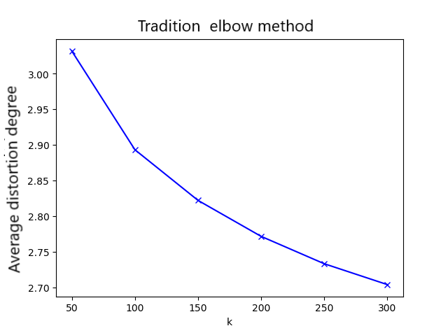
Improve the elbow method
Through a large number of experiments, it was found that due to the complexity of domain's surface shape information, the decline trend of using the elbow method was not obvious. However, just changing the key formula ingeniously can improve it significantly[6]:
The improved formula:
$S_{ET}=\sum \limits_{i=1}^{k}e\frac{\sum_{p\in C_{i}}\mid p-c_{i}\mid^{2}}{\theta}+e\frac{\underset{1<i<k}{max}\sum_{p\in C_{i}}\mid p-c_{i}\mid^{2}}{\varTheta}$
In this formula, $k$ is the number of clusters set artificially, $c_{i}$ is the center of the cluster $C_{i}$ ,and $\theta$ is the weight,which is responsible for adjusting the value of the sum of squared errors within the cluster $p$ is the sample point in the cluster $C_{i}$
Improved result:

It can be seen that the effect of improving the elbow rule is significant.
The proof of the number of clusters
In order to judge the accuracy of our clustering results, we also looked for a series of methods to prove it. After many experiments, we find that the silhouette coefficient is an ideal index, which can reasonably explain our classification results.
Silhouette coefficient
The silhouette coefficient[7] combines cohesion and separation. The calculation steps are as follows:
|
1. For the i-th object, we calculate the average distance from it to all other objects in the cluster, and record ai (reflecting the degree of cohesion) |
2. For the i-th object and any cluster that does not contain the selected object, we calculate the average distance between the object and all objects in the given cluster, and record bi (to reflect the degree of separation) |
|
3.The silhouette coefficient of the i-th object is si = (bi-ai)/max(ai, bi) |
$s(i)=\frac{b(i)-a(i)}{max\left\{ a(i),b(i)\right\} }$ $s(i)=\begin{cases} 1-\frac{a(i)}{b(i)}, & a(i)<b(i)\\ 0, & a(i)=b(i)\\ \frac{b(i)}{a(i)}-1, & a(i)>b(i) \end{cases}$
|
4.It can be seen from the above that the value of the silhouette coefficient is [-1, 1] ,.the larger the value, the better, and when the value is negative, it indicates that a(i) < b(i) , and the sample is allocated to the wrong cluster.That is to say, the clustering result is not acceptable. For results close to 0 , it indicates that the clustering results overlap. |

From the figure,we can draw a conclusion that clustering 100 is ideal.
Data preparation
RCSB PDB:
The GO functional database linked in PDB is adopted for protein functional crawling.This information shows how each chain of the protein is involved in the function of the protein.
After crawling, the functional information involved in the chain is counted. According to the protein chain where domain is located, the corresponding relation between each type and function is obtained.
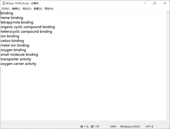
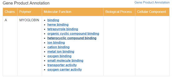
Obtain the functional label of the protein corresponding to the de-redundant domain in the GeneProduct Annotation database Geneontology .
After statistics, the function tag corresponding to each domain class and the frequency of each tag appearing in the structural class are obtained.
Extract function entries in each domain class where the frequency of function tags is higher than 10% and 20% respectively.
Take function items with a frequency of more than 20% as an example.
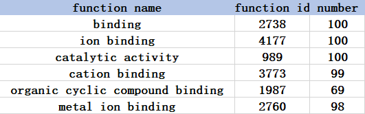
The go database parent node has a high degree of functional label redundancy.
Some function entry descriptions are too vague and occur more frequently than the threshold in almost all structure classes.
This part of function entry has very limited guidance for synthesis and is prone to misunderstanding. Therefore, based on function description and frequency, the above function labels are manually checked and deleted.
The function tag corresponding to each structure class is finally obtained.
Combined score
We used statistical methods to calculate the combined score according to the following formula
$P_{ij}=\frac{N_{ij}}{Nmax}\times10$
Where Nij is the number of domain pairs in the same protein in the i-th and j-th classes . (For example, in the traversal process, it is found that 101mA01 is in the i-th category, and 101mB02 is in the j-th category, then Nij+1 )
After calculating the number of combinations of each class with other classes, a 100*100 matrix N (100 matrix in total) is obtained, and Nmax is the maximum value of the entire 100*100 N matrix.Let the score of this combination be 10 points.The number of other combinations is linearly mapped to obtain a score Pij ranging from 0 to 10.
Model design strategy
This section is intended to further achieve domain prepare spliced entity, the derived model is mainly used for 3D printing Entity finished, by insertion of a cartridge at different locations solid interfaces now free splicing, color dependent on the electrical distribution model surface provided Clusters can be combined with actual depressions to determine a better binding position and visualize the free combination of structural domains.
The implementation steps are as follows:
|
1. According to the PDB files obtained in batches from the database and the distribution description of the structural domains, sort out the atomic information of the corresponding structural domains in the PDB file and only the atomic information. 
The picture above shows the atom information in the PDB . Columns 4 , 5 and 6 from right to left are the space coordinates of the atoms. 
The figure shows the distribution number of the structural domain corresponding to a certain PDBID in the chain. According to the above two parts, we can filter out the useful information in ATOM . |
2. Visualization . Dump the sorted ATOM information into a PDB file and import it into visualization software ( eg.PyMol , VMD , Chimera ), import PyMol here , define the charge color scheme, and export the VRML 2 (.wrl) file, and import it into Blender for further edit. |
3. In Blender changing the color for the vertex power distribution to see, in this embodiment the end portion similar to FIG. Next, create a connection port cartridge (cartridge after two dimensions defined Boolean intersection), the interface will be a certain distance into the Boolean model and the model modifier is added to the intersection with the interface, multiple treatments to obtain a final solution. |
Optimization Strategy
|
1. To improve processing efficiency and ensure the freedom of entity splicing, the number of interfaces is determined to be about 6. Create an interface in the positive and negative half-axis positions of the three-coordinate axis, and make small adjustments according to the actual recess. For the part of the interface close to the protrusion, you can set a new insertion direction to ensure normal splicing. |
2. In the previous scheme, it is considered that the interface placement process should be simplified regardless of whether the interface is determined according to the pocket calculation result. For this reason, relying on the bpy interface to design batch processing scripts. Both reading and interface placement are repeated or cyclic steps. In order to improve efficiency, it is recommended to place the interface in the positive direction of the x- axis, so that the model can always determine interest based on the input coordinates. Point, and automatically rotate the point to the positive x- axis direction to facilitate the direct connection of interfaces. The steps are repeated calling so it is omitted, here is an example of the rotation function. |
References
[1] Novotni M, Klein R. 3D Zernike Descriptors for Content Based Shape Retrieval[J]. 2003:216.
[2] La D, Juan Esquivel-Rodríguez, Venkatraman V, et al. 3D-SURFER: software for high- throughput protein surface compa rison and analysis[J]. Bioinformatics, 2009.
[3] Wang Jianren , Ma Xin , Duan Ganglong . Improved K-means clustering k value selection algorithm [J]. Computer Engineering and Applications , 2019, 55(08): 27-33.
[4] Han J, Kamber M. Data mining:Concepts and Techniques[M]. San Fromcisco:Morgan Kaufmann, 2006:483-486.
[5] Andrew Ng, Clustering with the K-Means Algorithm, Machine Learning, 2012
[6] MacQueen, J. Some Methods for Classification and An alysis of MultiVariate Observations[C]// Proc of Berkeley Symposium on Mathematical Statistics & Probability. 1965.
[7] Peter RJ. Silhouettes: A graphical aid to the interpretation and validation of cluster analysis[J]. Journal of Computational & Applied Mathematics, 1999, 20.