Team:ZJU-China/Model

Model
Overview
To understand the production of target antibody and modified magnetosomes and the combination and disaggregation of them, we have established some in-vivo and in-vitro models.
Our modeling work is comprised of three parts.
1) We used two models to describe the reactions in E.coli and magnetotactic bacteria separately.
2) We used a deterministic model to determine the combination and disaggregation of scFv-Fc and modified magnetosomes in vitro.
3) We used two models to describe the movements of modified magnetosomes and its combination with HER2 in vivo.
PART Ⅰ Deterministic Model to Compute the Production of scFv and Modified Magnetosomes
To produce scFv and modified magnetosomes, we introduced the plasmid containing target gene into E.coli and magnetotactic bacteria respectively, and finally understood the final yield of the target product by simulating their metabolic processes respectively.
E.coli
In E.coli, T7 RNA polymerase is placed under a lac Operon, which can be induced by IPTG. The production of the target protein, scFv-Fc, is controlled by T7 promoter (Figure 1)[1]. The combination between T7 RNA polymerase and T7 promoter is determined by Hill function. The ordinary differential equations (ODEs) describing these processes are shown as follows, and parameter names and chemical equations can be found in the appendix.
\begin{align} &\frac{d}{d t}MR_{E} = \alpha_MR \cdot O_{total} - \lambda_{MR} \cdot MR_{E}\\ &\frac{d}{dt}R_{E}=\beta_{R} \cdot MR_{E} -2 \cdot k_{2R} \cdot R_{E}^2 +2 \cdot k_{-2R} \cdot R_{2E} -\lambda_{R} \cdot R_{E}\\ &\frac{d}{dt}R_{2E}= 2 \cdot k_{2R} \cdot R_{E}^{2}-2 \cdot k_{-2R} \cdot R_{2E}-k_{r} \cdot R_{2 E} \cdot O_{E} +k_{-r} \cdot \left(O_{total}-O_{E}\right)-k_{dr1} \cdot R_{2E} \cdot I_{E}^{2} \\&\:\:\:\:\:\:\: + k_{-dr1} \cdot I_{2}R_{2E}-\lambda_{R2} \cdot R_{2E}\\ &\frac{d}{dt}O_{E}=-k_{r} \cdot R_{2E} \cdot O_{E}+k_{-r} \cdot \left(O_{total}-O_{E}\right)+k_{dr2} \cdot \left(O_{total}-O_{E}\right) \cdot I_{E}^{2}-k_{-dr2} \cdot O_{E} \cdot I_{2}R_{2E}\\ &\frac{d}{dt}I_{E}= -2 \cdot k_{dr1} \cdot R_{2E} \cdot I_{E}^{2} +2 \cdot k_{-dr1} \cdot I_{2}R_{2E}-2 \cdot k_{dr2} \cdot \left(O_{total}-O_{E}\right) \cdot I_{E}^{2} \\&+2 \cdot k_{-dr2} \cdot O_{E} \cdot I_{2}R_{2 E}+k_{ft} \cdot YI_{exE}+k_{t} \cdot \left(I_{ex}-I_{E}\right)+2 \cdot \lambda_{I2R2} \cdot I_{2}R_{2E}\\ &\frac{d}{dt}I_{2}R_{2E}=k_{dr1} \cdot R_{2E} \cdot I_{E}^{2} -k_{-dr1} \cdot I_{2}R_{2E} +k_{dr2} \cdot \left(O_{total}-O_{E}\right) \cdot I_{E}^{2} -k_{-dr2} \cdot O_{E} \cdot I_{2}R_{2E} \\&\:\:\:\:\:\:\:-\lambda_{I2R2} \cdot I_{2}R_{2E}\\ &\frac{d}{dt}MY_{E}=\alpha_{0} \cdot \left(O_{total}-O_{E}\right) +\alpha_{1} \cdot O_{E} -\lambda_{MY} \cdot MY_{E}\\ &\frac{d}{dt}Y_{E}=\beta_{Y} \cdot MY_{E}+\left(k_{ft}+k_{-p}\right) \cdot YI_{exE} -k_{p} \cdot Y_{E} \cdot I_{exE}-\lambda_{Y} \cdot Y_{E}\\ &\frac{d}{dt}YI_{exE}=-\left(k_{ft}+k_{-p}\right) \cdot YI_{exE}+k_{p} \cdot Y_{E} \cdot I_{exE} -\lambda_{YIex} \cdot YI_{exE}\\ &\frac{d}{dt}MT7_{E}=\alpha_{0} \cdot \left(O_{total}-O_{E}\right)+\alpha_{1} \cdot O_{E} -\lambda_{MT7} \cdot MT7_{E}\\ &\frac{d}{dt}pT7_{E}=\beta_{T7} \cdot MT7_{E}-\lambda_{pT7} \cdot pT7_{E}\\ &\frac{d}{dt}MF_{E}=\left(\frac{pT7^{n}}{pT7^{n}+K_{d}^{n}} \cdot \alpha_{MT}+\alpha_{leak}\right) \cdot O_{total}-\lambda_{MF} \cdot MF_{E}\\ &\frac{d}{dt}F_{E}=\beta_{F} \cdot MF_{E}-\lambda_{F} \cdot F_{E} \end{align}
According our modeling result, although there's a peak before adding IPTG, the production cannot be maintained during a long period of time. Only after adding IPTG, the concentration of the target protein in the bacteria is maintained at 1.3069×10⁴ nM.
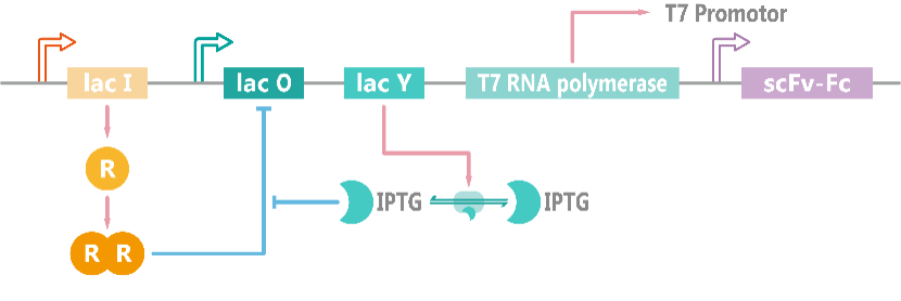
Figure 1. Schematic diagram of the induced expression model of scFv-Fc.
Figure 2. Dynamics of target protein. Horizontal axis shows the length of time. Vertical axis demonstrates the amount of protein (scFv-Fc) within the system.
Magnetotactic Bacteria
In magnetotactic bacteria, target protein (mamC-ZZ) is placed under a lac Opera, and the repressor protein LacI is stably expressed in the cell, two molecules of LacI will form a dimer which binds to LacO DNA fragment and represses the expression of target protein (Figure 3). When IPTG is added and transported into the cell, IPTG molecules will bind with LacI and inhibit its binding to LacO. In this way, target protein can be rescued from suppression[1]. We assume that all target proteins will be localized to the magnetosome membrane by intracellular transport. The ordinary differential equations (ODEs) describing these processes are shown as follows, parameter names and chemical equations can be found in the appendix.
\begin{align} &\frac{d}{d t}MR_{M}= \alpha_MR \cdot O_{total} - \lambda_{MR} \cdot MR_{M}\\ &\frac{d}{dt}R_{M}=\beta_{R} \cdot MR_{M} -2 \cdot k_{2R} \cdot R_{M}^2 +2 \cdot k_{-2R} \cdot R_{2M} -\lambda_{R} \cdot R_{M}\\ &\frac{d}{dt}R_{2M}=2 \cdot k_{2R} \cdot R_{M}^{2}-2 \cdot k_{-2R} \cdot R_{2M}-k_{r} \cdot R_{2M} \cdot O_{M} +k_{-r} \cdot \left(O_{total}-O_{M}\right)-k_{dr1} \cdot R_{2M} \cdot I_{M}^{2} \\&\:\:\:\:\:\:\:+k_{-dr1} \cdot I_{2}R_{2M}-\lambda_{R2} \cdot R_{2M}\\ &\frac{d}{dt}O_{M}=-k_{r} \cdot R_{2M} \cdot O_{M}+k_{-r} \cdot \left(O_{total}-O_{M}\right)+k_{dr2} \cdot \left(O_{total}-O_{M}\right) \cdot I_{M}^{2}-k_{-dr2} \cdot O_{M} \cdot I_{2}R_{2M}\\ &\frac{d}{dt}I_{M}=-2 \cdot k_{dr1} \cdot R_{2M} \cdot I_{M}^{2} +2 \cdot k_{-dr1} \cdot I_{2}R_{2M}-2 \cdot k_{dr2} \cdot \left(O_{total}-O_{M}\right) \cdot I_{M}^{2} \\&+2 \cdot k_{-dr2} \cdot O_{M} \cdot I_{2}R_{2M}+k_{ft} \cdot YI_{exM}+k_{t} \cdot \left(I_{ex}-I_{M}\right)+2 \cdot \lambda_{I2R2} \cdot I_{2}R_{2M}\\ &\frac{d}{dt}I_{2}R_{2M}=k_{dr1} \cdot R_{2M} \cdot I_{M}^{2} -k_{-dr1} \cdot I_{2}R_{2M} +k_{dr2} \cdot \left(O_{total}-O_{M}\right) \cdot I_{M}^{2} -k_{-dr2} \cdot O_{M} \cdot I_{2}R_{2M} \\&\:\:\:\:\:\:\:-\lambda_{I2R2} \cdot I_{2}R_{2M}\\ &\frac{d}{dt}MY_{M}=\alpha_{0} \cdot \left(O_{total}-O_{M}\right) +\alpha_{1} \cdot O_{M} -\lambda_{MY} \cdot MY_{M}\\ &\frac{d}{dt}Y_{M}=\beta_{Y} \cdot MY_{M}+\left(k_{ft}+k_{-p}\right) \cdot YI_{exM} -k_{p} \cdot Y_{M} \cdot I_{exM}-\lambda_{Y} \cdot Y_{M}\\ &\frac{d}{dt}YI_{exM}=-\left(k_{ft}+k_{-p}\right) \cdot YI_{exM}+k_{p} \cdot Y_{M} \cdot I_{exM} -\lambda_{YIex} \cdot YI_{exM}\\ &\frac{d}{dt}MZ_{M}=\alpha_{0} \cdot \left(O_{total}-O_{M}\right)+\alpha_{1} \cdot O_{M} -\lambda_{MZ} \cdot MZ_{M}\\ &\frac{d}{dt}Z_{M}=\beta_{Z} \cdot MZ_{M}-\lambda_{Z} \cdot Z_{M} \end{align}
According to our modeling result, the final concentration of target protein mamC-ZZ is 2.3625×10³ nM. Since the concentration of magnetosomes extracted from the culture medium whose OD600 reaches 1 is 172 ug per milliliter[2], the average concentration of magnetosomes is 46.83 per cell, and there are an average of 24.31 target protein mamC-ZZ on each magnetosome when assuming that all target proteins are localized to the magnetosome membrane.
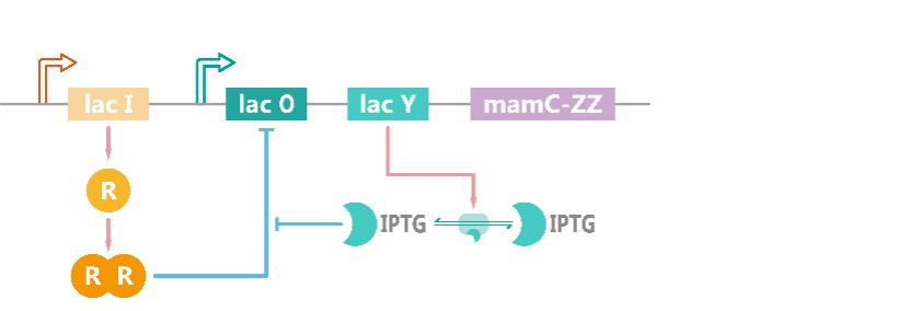
Figure 3. Schematic diagram of the model of induced expression of mamC-ZZ.
Figure 4. Dynamics of target protein. Horizontal axis shows the length of time. Vertical axis demonstrates the amount of protein (mamC-ZZ) within the system.
PART Ⅱ Deterministic Model to Determine the Combination and Disaggregation of scFv-Fc and Modified Magnetosomes in Vitro
After scFv-Fc and modified magnetosomes being produced in E.coli and magnetotactic bacteria, they are extracted from cells and purified Fc domain can combine with mamC-ZZ domain so that these two parts will combine and work together. Assuming that there's no factor causing target protein degradation in vitro, the ordinary differential equations (ODEs) describing these processes are shown as follows.
$$\frac{d}{dt}F=-k_{1} \cdot F \cdot Z+k_{-1} \cdot FZ$$ $$\frac{d}{dt}Z=-k_{1} \cdot F \cdot Z+k_{-1} \cdot FZ$$ $$\frac{d}{dt}FZ=k_{1} \cdot F \cdot Z-k_{-1} \cdot FZ$$
From the modeling result, we can see the reaction between 10 mg/ml modified magnetosomes and 100 ug/ml scFv-Fc is very fast and the production rate is relatively high (Figure 5).
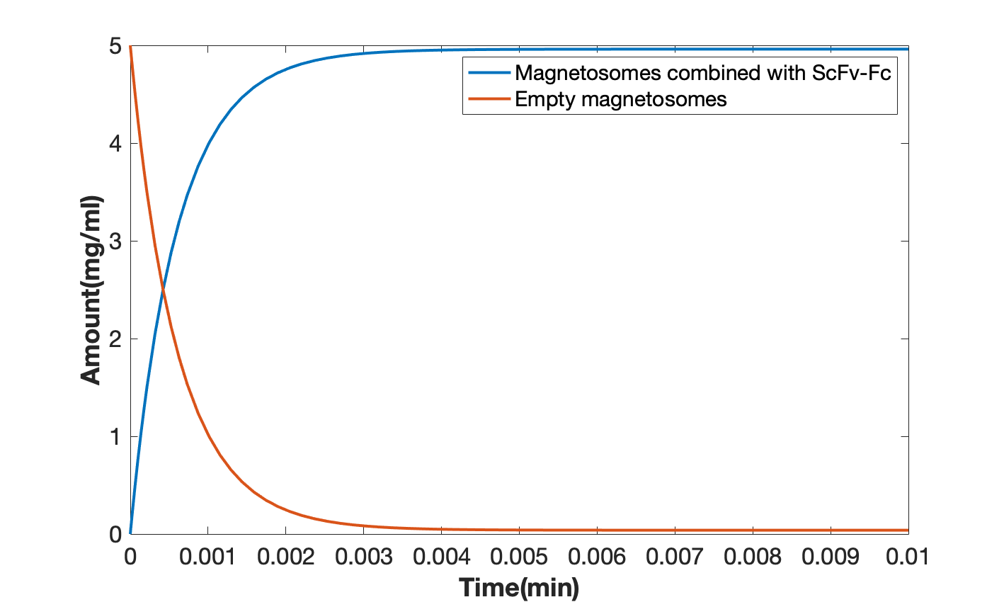
Figure 5. combination of scFv-Fc and modified magnetosomes (the blue line refers to the combination product of scFv-Fc and modified magnetosomes, and the orange line refers to pure magnetosomes).
PART Ⅲ Kinetic Model to Simulate the Diffusion and Binding of Modified Magnetosomes Inside the Tumors
Magnetosome Diffusion in Internal Environment
It could be assumed that the magnetosome injected collect around the tumor if exists, since our magnetosome has been proved to stick to HER2 produced by breast cancer cells specifically. As magnetosome enters into tissue fluid from blood, its concentration changes with time and the distance to the source. This way, we want to depict the alteration of magnetosome's concentration field to explain the process intuitively by image.
First of all, we'd like to focus on the factors which drive magnetosome move or diffuse in tissue fluid. Four respects were considered, involving motions with the flow of tissue fluid, eddy diffusion caused by natural convection, mass transfer due to the difference of concentration, pure molecular diffusion as magnetosome was regarded as similar to a molecular in size.
To simplify the question, polar coordinates were adopted to substitute a two-dimension or three-dimension gradient. That is to say, small particles were assumed to diffuse evenly to different directions and scalars were calculated instead of vectors.
$$\nabla \boldsymbol{c} \rightarrow \frac{\partial c}{\partial r}$$
Macroscopic methods could be useful to solve the problem. Use J to represent the diffusion flux. It is easy to infer motions with the flow of tissue fluid as \(J_{1}=ub \times \frac{\partial c}{\partial r}\\\).
$$u_{b}=\frac{\pi d^{2}\left(p+\frac{1}{2} \rho g d\right)}{32 \mu_{b} D}$$
According to Fick's First Law, eddy diffusion caused by natural convection is calculated by \(J_{2}=D_{n} \times \frac{\partial c}{\partial r}\\\).
On top of that, natural convection is very weak in both capillaries and tissue fluid flows. We chose to ignore the value of J2 finally, which means \(J_{2} \approx 0\\\).
In order to obtain the diffusion flux due to mass transfer, an important constant called mass transfer coefficient was in need, for the expression, \(J_{3}=k_{c} \times \frac{\partial c}{\partial r}\\\).
We used Chaoqun Yao (2020)'s experiment kc data of 1:1 silicone oil-water mixture, to whose viscosity blood and tissue fluid similar[3]. A model was built for the relationship between the rate of flow and kc. Microsoft Office Excel was employed to finish the task.
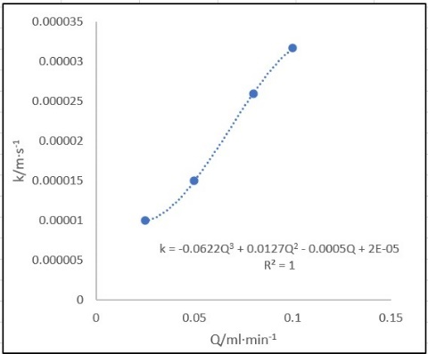
Figure 6. The influence of rate of flow on mass transfer coefficient.
Now we could get the value of Q in our situation. This way, the value of kc could be assumed roughly.
$$Q=u_{a} \times \frac{1}{4} \pi d^{2}=4.01 \times 10^{-4} ml/min$$ $$k_{c}=-0.0622 Q^{3}+0.0127 Q^{2}-0.0005 Q+2 \times 10^{-5}=2.00 \times 10^{-2} mm/s$$
Dispersion effect also led to the diffusion of magnetosome in tumor tissue. It could be estimated the same way as eddy diffusion caused by natural convection:
$$J_{4}=D_{m} \times \frac{\partial c}{\partial r}$$
Stokes-Einstein equation was able to be used to calculate the diffusion coefficient as below.
$$D_{m}=\frac{k_{b} T}{6 \pi \mu_{b} R}$$
Overall diffusion flux could be calculated by superimposing the following diffusion flux.
$$J=J_{1}-J_{2}-J_{3}-J_{4}$$
It is assumed that the motion of fluid flow obeys the law discovered by Navier and Stokes.
instantaneous term = - diffusion term + convection term + sourse
That is to say,
$$\frac{\partial c}{\partial t}=\frac{\partial J}{\partial r}+u_{a} \nabla \boldsymbol{c}_{\boldsymbol{o}}$$
To solve the following PDE with the help of MatlabR2020a, both initial condition and boundary condition were supposed to be provided.
We should provide the relationship between r and c under the circumstance that t–0, when diffusion hadn't happened in our model. At the very beginning, magnetosome collect in the capillary and it is presumed that there was seldom magnetosome in tissue fluid.
$$ \left.c(t, r)\right|_{t=0}=\left\{\begin{array}{ll} 0 & r \neq 0 \\ c_{o} & r=0 \end{array}\right. $$
In comparison to the initial condition, this time we're required to explain how t influences c at the time of rmin=0 and rmax=10, embodying the probable size of the tumor. Soon we found the condition invalid. At last we expand rmax=100 to produce the image.
One of the difficulties was that we failed to describe the alteration of the concentration taking place at the original location where diffusion started precisely and in detail. A highly rough calculation was attached to it to show the characteristics that the rate of diffusion weakened as the concentration descended and time went by.
$$\left.c(t, r)\right|_{r=0}=\frac{c_{o}}{1+0.05 \sqrt{t}}$$
Simultaneously, we assumed that when diffusion flux caught the brim space, co would be small enough to be ignored.
$$\left.c(t, r)\right|_{r=100}=0$$
Figure 7. Concentration field of magnetosome in tissue fluid.
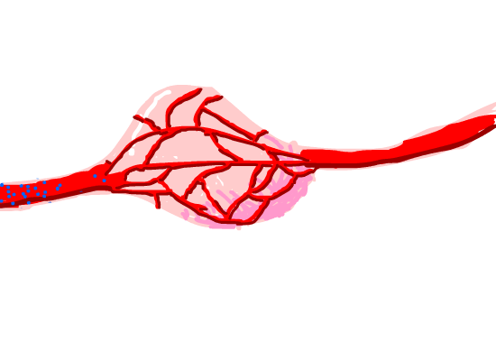
Figure 8. Magnetosome diffused in the tumor issue capillaries around it.
Detection and Combination with HER2
To describe the combination and degradation with HER2, we have a model about modified magnetosomes in vivo. Assuming that there is no other way to clear magnetosomes and scFv-Fc in the tissue fluid except for phagocytosis by macrophages and the phagocytosis is at a constant rate, the ordinary differential equations (ODEs) describing these processes are as follows. Parameter names and chemical equations can be found in the appendix.
$$\frac{d}{dt}F=-k_{1} \cdot F \cdot Z+k_{-1} \cdot FZ -k_{2} \cdot H \cdot F +k_{-2} \cdot FH$$ $$\frac{d}{dt}Z=-k_{1} \cdot F \cdot Z+k_{-1} \cdot FZ -k_{1} \cdot FH \cdot Z+k_{-1} \cdot ZFH-P$$ $$\frac{d}{dt}FZ=k_{1} \cdot F \cdot Z-k_{-1} \cdot FZ -k_{2} \cdot H \cdot FZ+k_{-2} \cdot ZFH-P$$ $$\frac{d}{dt}H=-k_{2} \cdot H \cdot F+k_{-2} \cdot FH -k_{2} \cdot H \cdot FZ+k_{-2} \cdot ZFH$$ $$\frac{d}{dt}FH=k_{2} \cdot H \cdot F-k_{-2} \cdot FH -k_{1} \cdot FH \cdot Z+k_{-1} \cdot ZFH$$ $$\frac{d}{dt}ZFH=k_{1} \cdot FH \cdot Z-k_{-1} \cdot ZFH+k_{2} \cdot H \cdot FZ-k_{-2} \cdot ZFH$$
We can see in the result that the process of combination finished very quickly (Figure 9A), while the total number of the magnetosomes decreases gradually because of the phagocytosis process (Figure 9B), and the concentration of magnetosomes is one tenth of what it was before after around 120 minutes. We also have results with different concentration of magnetosomes injected (Figure 9C), which shows the combination in a short of time with different injection concentration of modified magnetosomes.
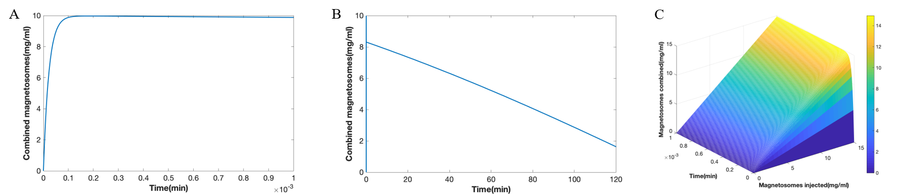
Figure 9. (A) Magnetosome binding in a short time. (B) Metabolism of magnetosomes in the body for a long time. (C) The combination of different concentrations of magnetosomes in a short time after injection.
Appendix
Please consult the following file for a clearer understanding of the formulation of the model.
References
[1]. Stamatakis, M., & Mantzaris, N. V. (2009). Comparison of deterministic and stochastic models of the lac operon genetic network. Biophysical journal, 96(3), 887–906. https://doi.org/10.1016/j.bpj.2008.10.028
[2]. Xiang, L., Wei, J., Jianbo, S., Guili, W., Feng, G., & Ying, L. (2007). Purified and sterilized magnetosomes from Magnetospirillum gryphiswaldense MSR-1 were not toxic to mouse fibroblasts in vitro. Letters in applied microbiology, 45(1), 75–81. https://doi.org/10.1111/j.1472-765X.2007.02143.x
[3]. Yao, C., Ma, H., Zhao, Q., Liu, Y., Zhao, Y., & Chen, G. (2020). Mass transfer in liquid-liquid Taylor flow in a microchannel: Local concentration distribution, mass transfer regime and the effect of fluid viscosity. Chemical Engineering Science, 223, 115734. https://doi.org/10.1016/j.ces.2020.115734
