Team:GunnVistaPingry US/Model

Model

Machine learning for better sgRNA prediction

• Training and test datasets
• Features
• Transformation process
• Calculating features
• Method
• Findings
• Discussion
• Scatter plots
• Flowchart
• Limitations

Training and test datasets

The CRISPRi activity dataset with 190 records of 18 genes was provided by Dr. Samuel Perli (who works at Yamanaka lab in Gladstone Institute, UCSF) to build the regression model. 10 records of ‘EIF4G1’ gene were set aside as test/validation dataset and remaining 180 records were used to train the data model.

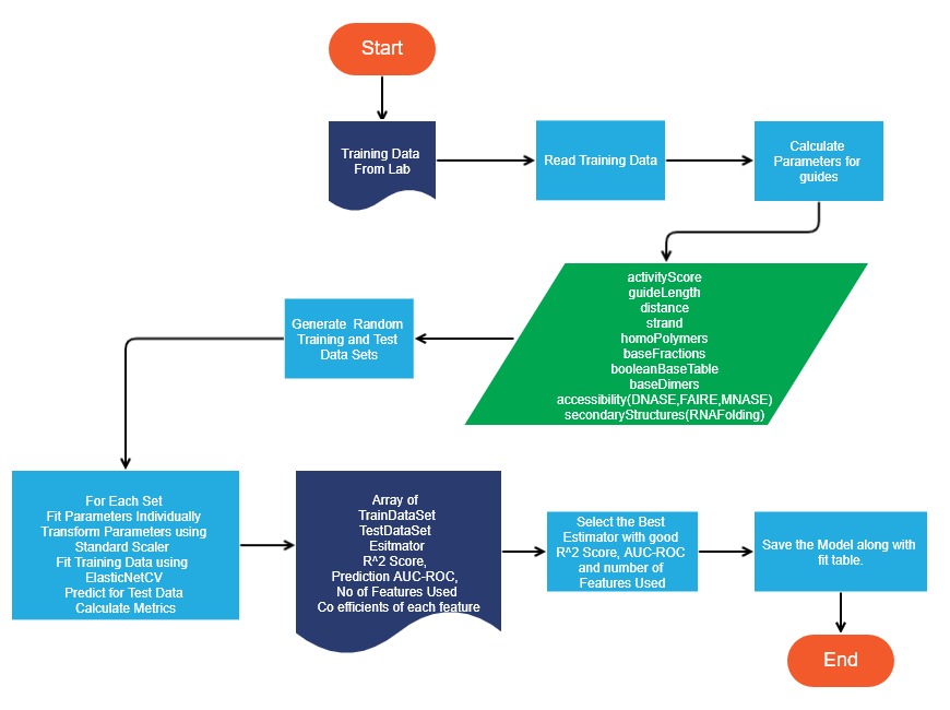
The training data set was randomly divided into 17 gene folds where each fold has a further distribution of 94% and 6% for training and test data sets, respectively.

y = w₀x₀ + w₁x₁ + w₂x₂ + w₃x₃ + w₄x₄ + ................. +w_nx_n

y -- Score of the Guide
w₀ ... w_n -- Weights of features contributing to score
x₀ ... x_n -- Features contributing to score as predicted by the algorithm.

Features

The model was trained with below features that would affect the activity score of sgRNA. However, as most of the features were nonlinear with activity score, a transformation process was required prior to linear regression.

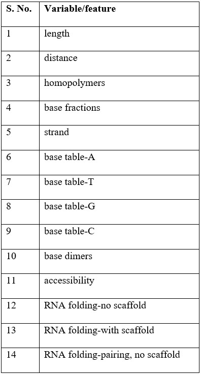
Table-1: List of variables/features

Transformation process[1]

Each feature set was adapted according to its relationship with activity score and categorical & non-linear parameters were binned. After analyzing the relationship between lab scores vs distance of sgRNA from TSS, we added square of the distance as additional parameter [refer the scatter plots section at the end for further explanation. Features that contributed the most to CRISPRi activity score were analyzed in the predictive model and it turned out the scores were most influenced by the square of the distance of sgRNA from TSS. This was a very key finding of this project.

Parameters were binned by a fixed width for each feature and applied over the range of values, with the upper-most and lower-most bins collapsed with the neighboring bins if the number of data points at each edge were sparse.

For binning parameters, a fixed-width was chosen for each feature/parameter and applied over the range of values, with the upper-most and lower-most bins collapsed with the neighboring bins if the number of data points at each edge were sparse. Each feature was then split into individual parameters for each bin and sgRNAs were assigned a 1 for the bin if the value fell within the bin or 0 if not. For linearizing sgRNA positioning parameters with continuous curves, sgRNA positions were fit to the activity score (individually for the distance to each TSS coordinate) using SVR with a radial basis function kernel and hyperparameters C and gamma determined using a grid search approach cross-validated within the training set. The fit score at each position was then used as the transformed linear parameter. Binary parameters were assigned a 1 if true or a 0 if false. All linearized parameters were z-standardized and fit with elastic net linear regression, with different L1/L2 ratio values [.5, .75, .9, .99, 1] as suggestions.

Calculating features[2]

The genomic coordinate of the PAM’s 3’G for each sgRNA to the upstream and downstream edge of each TSS range was used to calculate the position relative to the primary and secondary TSSs. Custom Python scripts with Biopython module were used to determine sequence features of the sgRNA and target sites.

ViennaRNA package was used with default parameters to calculate RNA folding metrics. The signal at each base of the target site including the PAM was averaged to calculate the chromatin features. Bx-python module was used to extract the processed continuous signal from the following BigWig files obtained from the ENCODE Consortium: MNase-seq https://www.encodeproject.org/files/ENCFF000VNN/ (Michael Snyder lab, Stanford University), DNase-seq https://www.encodeproject.org/files/ENCFF000SVY/ (Gregory Crawford lab, Duke University), and FAIRE-seq https://www.encodeproject.org/files/ENCFF000TLU/ (Jason Lieb lab, University of North Carolina) (ENCODE Project Consortium, 2012).

Method

The above transformation process^[1] translates the top-level features into low-level variables/features which were calculated^[2], linearized and z-standardized.

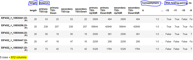
Fig-1: The top-level feature “distance” was translated into 8 low-level features: primary and secondary upstream/downstream normal distances & squares of distances from TSS

Each gene fold was then passed on to ElasticNetCV linear regressor [https://scikit-learn.org/stable/modules/generated/sklearn.linear_model.ElasticNetCV.html] and fit method was run.

Note: ElasticNetCV is a combination of Lasso and Ridge regressions. Lasso takes care of data set’s collinearity issues and ridge makes sure the regression model is not overfitted.

Findings

The coefficient R 2 values of all the 17 regression models were compared and the one with 0.24075410912510598 turned out to be the best, wherein the selected features/parameters were explaining 24% variance of activity score.

Note: The coefficient R^2 is defined as (1 - u/v), where u is the residual sum of squares ((y_true - y_pred) ** 2).sum() and v is the total sum of squares ((y_true - y_true.mean()) ** 2).sum(). The best possible score is 1.0 and it can be negative (because the model can be arbitrarily worse). A constant model that always predicts the expected value of y, disregarding the input features, would get a R^2 score of 0.0.
[https://scikit-learn.org/stable/modules/generated/sklearn.linear_model.ElasticNetCV.html]

As per the linear model that was generated, the following features (Table-1) contributed to the target activity score with corresponding coefficients (Fig-2).

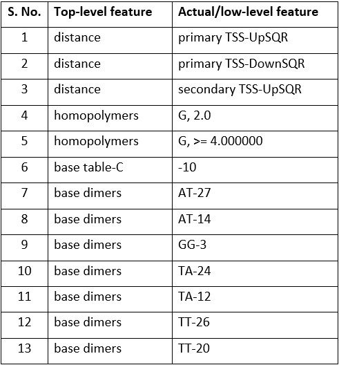
Table-2: Low-level variables/features of regression model with highest R 2 value.

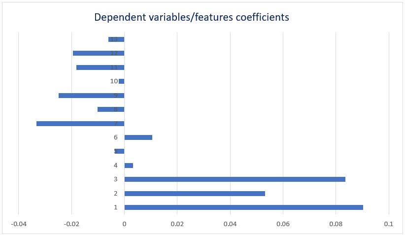
Fig-2: Coefficients of low-level variables/features of regression model with highest R 2 value.

Discussion

When the linear regression model with the highest coefficient R 2 value was used to predict the sgRNA scores for the ‘EIF4G1’ gene, the scores were closer to the lab scores when compared to the scores predicted by Weissman lab’s algorithm. A similar observation was found with other sgRNAs for which lab scores were known. So, it proves that even though our dataset was small, our model was predicting the scores well because of the data quality used. This algorithm can further be improved by training it with a larger dataset of scores measured using the qRT-PCR mechanism.
Click here for the results.

Scatter plots

Our improvement to Weissman lab’s study was the use of quality lab data and the inclusion of 4 low-level variables/features: Squares of primary and secondary upstream/downstream distances from TSS (Transcription Start Site) to guide. The reason for inclusion was, as we can see in the below scatter plots, the relationship between the scores and normal primary/secondary upstream/downstream distances from TSS was non-linear. The graphs looks like parabolas.

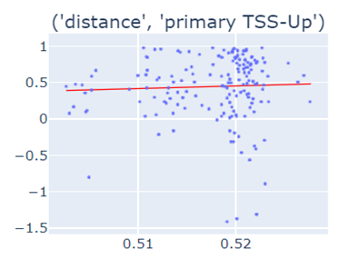
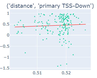
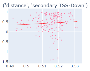
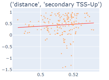
Fig-3: Scatter plots of primary/secondary upstream/downstream distances from TSS vs our algorithm score.

However, when we used squares of primary/secondary upstream/downstream distances from TSS to guide, we identified a strong & clear linear relationship.

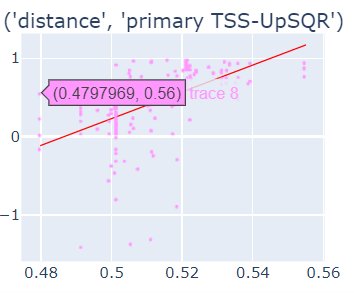
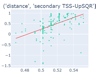
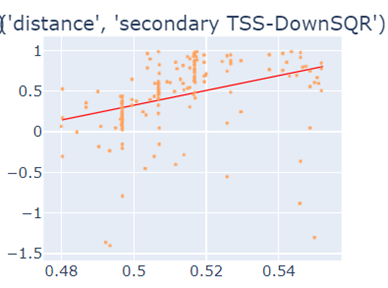
Fig-4: Scatter plots of squares of primary/secondary upstream/downstream distances from TSS vs our algorithm score.

Model Generator Flowchart

Limitations

• Availability of large quantity of qRT-PCR training data is difficult to obtain than phenotype based data
• Model is trained based on human genome hg19

Acknowledgment: Our model was inspired from https://elifesciences.org/articles/19760 research paper. We extend our sincere gratitude to all the authors & contributors of the paper.

Contact: navya.lavina@gmail.com For more info please visit ODIGOS website